Creating A Pie Chart In Excel
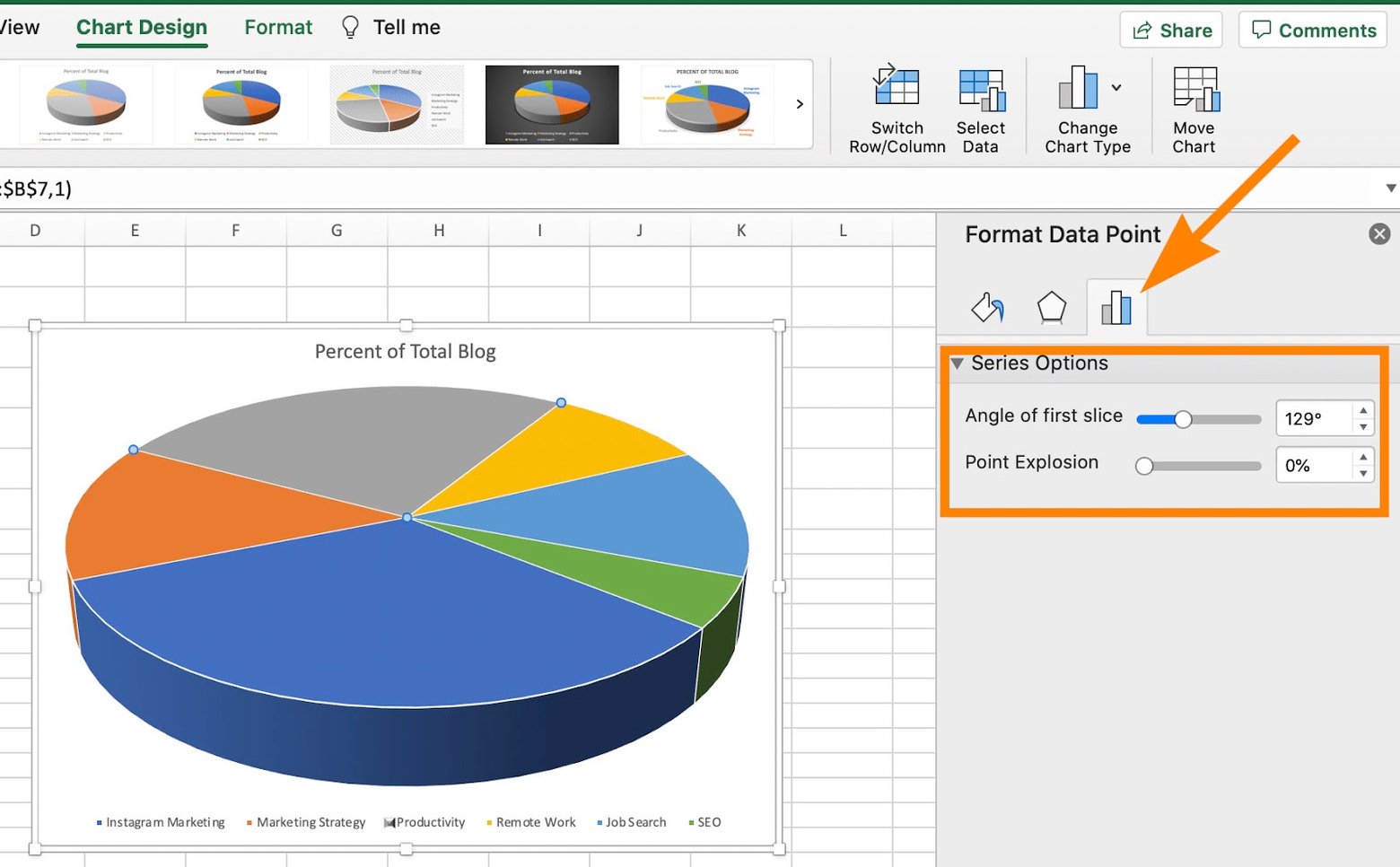
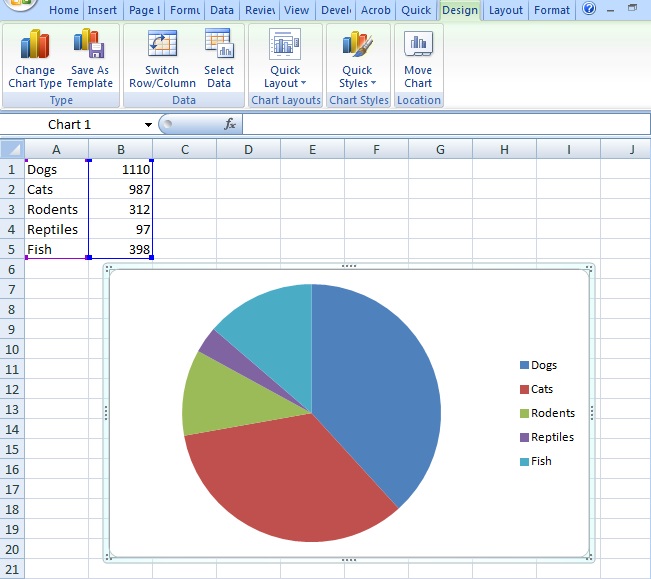
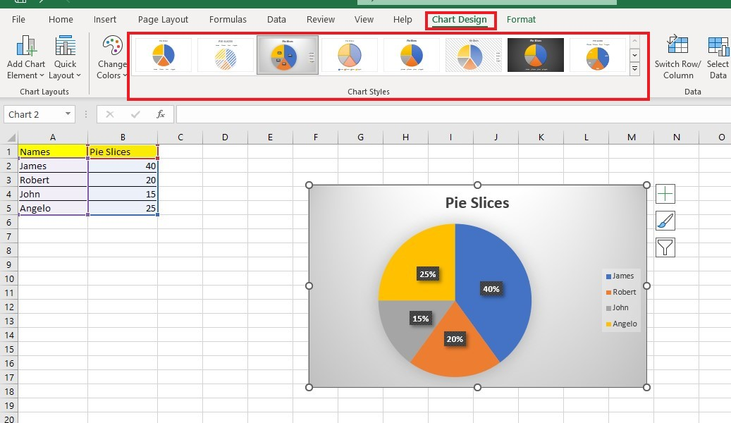
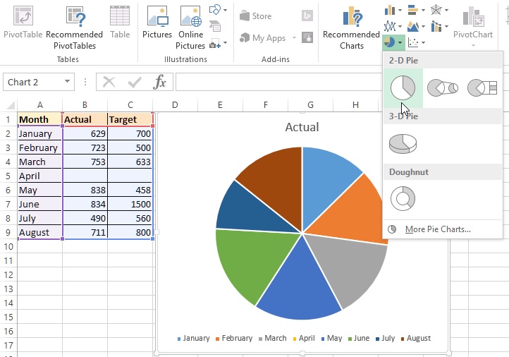
Creating A Pie Chart In Excel - Select insert > chart > pie and then pick the pie chart you want to add to your slide. Visualize your data with a column, bar, pie, line, or scatter chart (or graph) in office. To create a pie or doughnut chart (to show a proportion of a whole when your total equals 100%), press q. To select the type of the pie or doughnut chart, use the down arrow key and the. To customize the chart layout , select property sheet, set legend position to right and set chart title to order amount. But how do you communicate this visual information to people with low vision? For example, in the pie chart below, without the data labels it would. Using microsoft excel, you can quickly turn your data into a doughnut chart, and then use the new formatting features to make that doughnut chart easier to read. Data labels make a chart easier to understand because they show details about a data series or its individual data points. In the spreadsheet that appears, replace the placeholder data with your own information. But how do you communicate this visual information to people with low vision? To create a pie or doughnut chart (to show a proportion of a whole when your total equals 100%), press q. Learn best ways to select a range of data to create a chart, and how that data needs to be arranged for specific charts. To select the type of the pie or doughnut chart, use the down arrow key and the. Create a pivotchart based on complex data that has text entries and values, or existing pivottable data, and learn how excel can recommend a pivotchart for your data. Learn how to create a chart in excel and add a trendline. For example, in the pie chart below, without the data labels it would. Select insert > chart > pie and then pick the pie chart you want to add to your slide. In the spreadsheet that appears, replace the placeholder data with your own information. To make parts of a pie chart stand out without changing the underlying data, you can pull out an individual slice, pull the whole pie apart, or enlarge or stack whole sections by using a pie or. Learn best ways to select a range of data to create a chart, and how that data needs to be arranged for specific charts. To make parts of a pie chart stand out without changing the underlying data, you can pull out an individual slice, pull the whole pie apart, or enlarge or stack whole sections by using a pie. Using microsoft excel, you can quickly turn your data into a doughnut chart, and then use the new formatting features to make that doughnut chart easier to read. Learn how to create a chart in excel and add a trendline. To make parts of a pie chart stand out without changing the underlying data, you can pull out an individual. Learn how to create a chart in excel and add a trendline. Visualize your data with a column, bar, pie, line, or scatter chart (or graph) in office. Select insert > chart > pie and then pick the pie chart you want to add to your slide. For example, in the pie chart below, without the data labels it would.. Learn best ways to select a range of data to create a chart, and how that data needs to be arranged for specific charts. Create a pivotchart based on complex data that has text entries and values, or existing pivottable data, and learn how excel can recommend a pivotchart for your data. But how do you communicate this visual information. The charts and graphs you create in excel help make complex information easier to understand. In the spreadsheet that appears, replace the placeholder data with your own information. To create a pie or doughnut chart (to show a proportion of a whole when your total equals 100%), press q. To select the type of the pie or doughnut chart, use. Using microsoft excel, you can quickly turn your data into a doughnut chart, and then use the new formatting features to make that doughnut chart easier to read. The charts and graphs you create in excel help make complex information easier to understand. To make parts of a pie chart stand out without changing the underlying data, you can pull. In the spreadsheet that appears, replace the placeholder data with your own information. Learn how to create a chart in excel and add a trendline. Learn best ways to select a range of data to create a chart, and how that data needs to be arranged for specific charts. To make parts of a pie chart stand out without changing. Visualize your data with a column, bar, pie, line, or scatter chart (or graph) in office. To create a pie or doughnut chart (to show a proportion of a whole when your total equals 100%), press q. Select insert > chart > pie and then pick the pie chart you want to add to your slide. But how do you. Learn best ways to select a range of data to create a chart, and how that data needs to be arranged for specific charts. The charts and graphs you create in excel help make complex information easier to understand. In the spreadsheet that appears, replace the placeholder data with your own information. Select insert > chart > pie and then. Visualize your data with a column, bar, pie, line, or scatter chart (or graph) in office. Using microsoft excel, you can quickly turn your data into a doughnut chart, and then use the new formatting features to make that doughnut chart easier to read. In the spreadsheet that appears, replace the placeholder data with your own information. Data labels make. To make parts of a pie chart stand out without changing the underlying data, you can pull out an individual slice, pull the whole pie apart, or enlarge or stack whole sections by using a pie or. To customize the chart layout , select property sheet, set legend position to right and set chart title to order amount. Create a pivotchart based on complex data that has text entries and values, or existing pivottable data, and learn how excel can recommend a pivotchart for your data. But how do you communicate this visual information to people with low vision? To select the type of the pie or doughnut chart, use the down arrow key and the. Select insert > chart > pie and then pick the pie chart you want to add to your slide. Learn best ways to select a range of data to create a chart, and how that data needs to be arranged for specific charts. To create a pie or doughnut chart (to show a proportion of a whole when your total equals 100%), press q. Learn how to create a chart in excel and add a trendline. Data labels make a chart easier to understand because they show details about a data series or its individual data points. In the spreadsheet that appears, replace the placeholder data with your own information. Using microsoft excel, you can quickly turn your data into a doughnut chart, and then use the new formatting features to make that doughnut chart easier to read.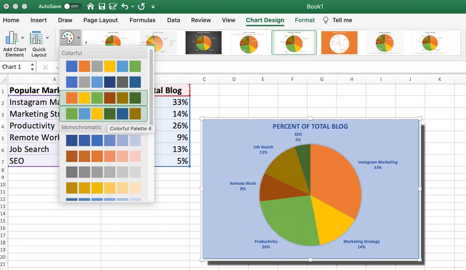
How to Create a Pie Chart in Excel in 60 Seconds or Less
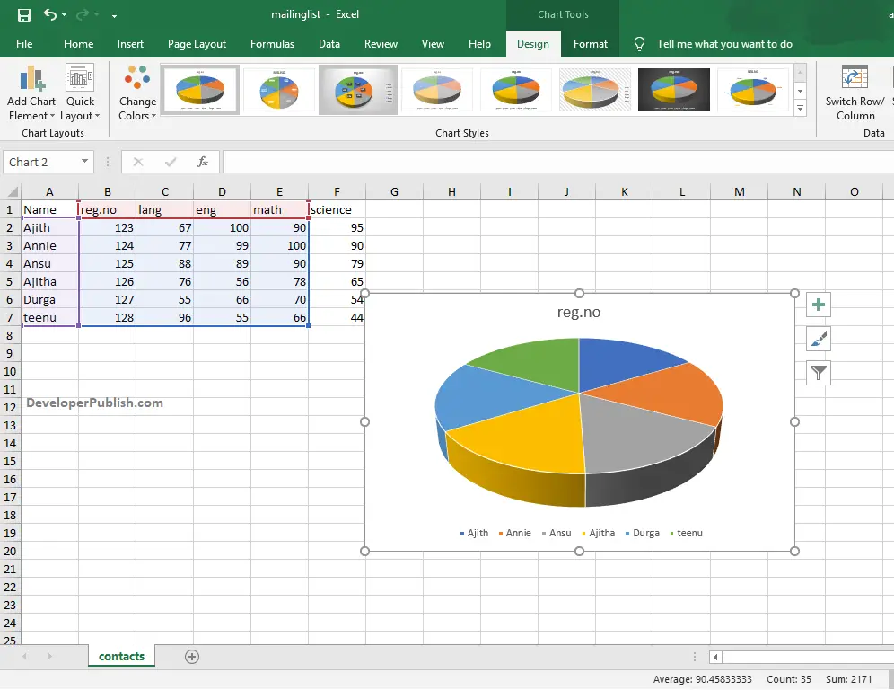
Pie Chart in Excel DeveloperPublish Excel Tutorials
Create A Pie Chart Excel How To Make A Pie Chart In Excel
How to Create a Pie Chart in Excel in 60 Seconds or Less
Pie Chart Definition, Examples, Make one in Excel/SPSS Statistics How To
How To Make A Pie Chart In Excel Everything You Need To Know

How to Make a Pie Chart in Excel 7 Steps (with Pictures)

How to Make Pie Chart in Excel with Subcategories (2 Quick Methods)
How To Create A Pie Chart In Excel (With Percentages) YouTube
How To Create A Pie Chart In Excel Ponasa
Visualize Your Data With A Column, Bar, Pie, Line, Or Scatter Chart (Or Graph) In Office.
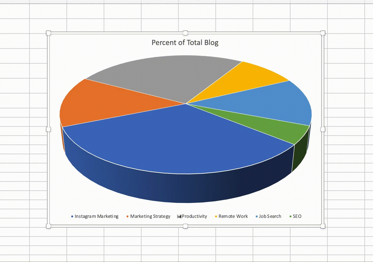
The Charts And Graphs You Create In Excel Help Make Complex Information Easier To Understand.
For Example, In The Pie Chart Below, Without The Data Labels It Would.
Related Post: